Note: Forcing dark mode via a plugin will make some pictures ugly (ironic because I do this). Sorry.
E-graphs are a cool data structure, but I think that what makes them cool also has the side effect of making them a little inscrutable.
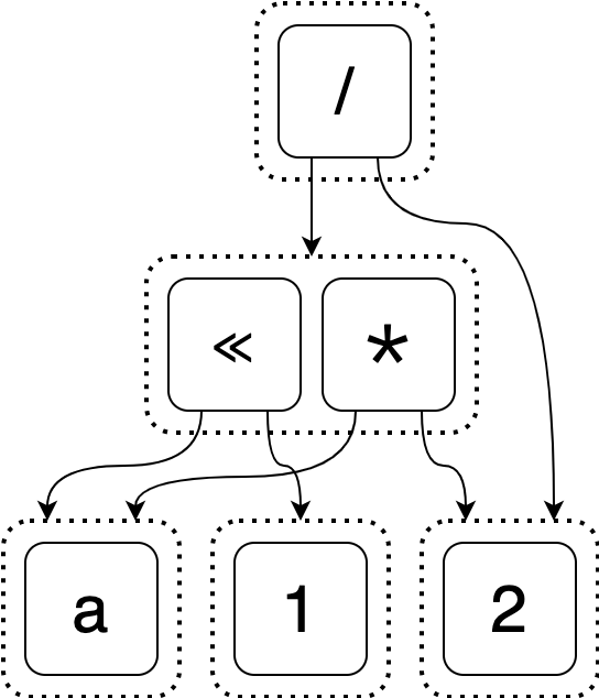
This is an e-graph.
Does it confuse you? It certainly took me a long time before I understood one.
My goal with this post is to
- Motivate two distinguishing features of e-graphs. (Section 1)
- Explain the e-graph data structure. (Section 2)
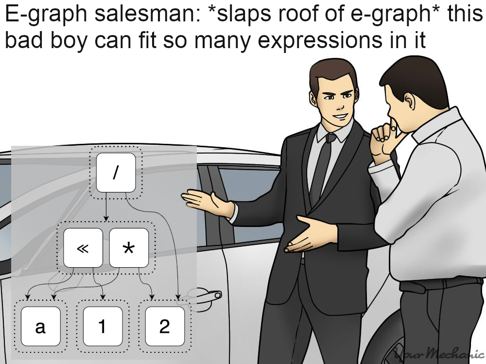
I’ve tried pretty hard to keep my explanations high-level and example-driven. Images comprise about half of the admittedly intimidating vertical height of this post (footnotes are another eighth). And I’ve tried to break up the monotony of dry, technical writing with some fun content.
I of course expect no prior knowledge of e-graphs!
I hope to convince you that e-graphs are cool and to make you comfortable reading and interpreting ones like the above and this one.
Section 1: Building up to the e-graph
In this section we will introduce an expression optimization problem and incrementally improve upon its naive solution. These improvements will eventually lead us to an e-graph.
The problem setting: expression optimization
In expression optimization, we want to take a (possibly naive) expression and generate an equivalent one that is more optimal. For simplicity, we’ll say that shorter expressions are better, but we could use other heuristics too.1
We will also narrow the scope of the problem by requiring that all the ways we can rewrite our expression are given to us in the form of rewrite rules. A rewrite rule says how we can transform our expression into another equivalent expression.2 An example is
x * 1 => x
and we can interpret it as saying that if we have part of our expression that
matches x * 1, we can generate an equivalent expression by replacing this part
with x. The arrow in the rewrite rule means you can only apply it forward (so
you can’t transform any x into x * 1).
For example, applying this rewrite rule twice will make the expression
(a + (3 * 1)) * 1
into
a + 3
(Not sure why this is the case? Read this footnote 3)
So to summarize: we are given an expression and some rewrite rules and our goal is to apply these rules to find the best (shortest) equivalent expression.
Our example
Our example expression, which I will refer back to throughout this post, is
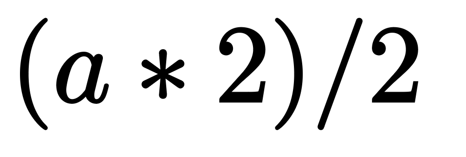
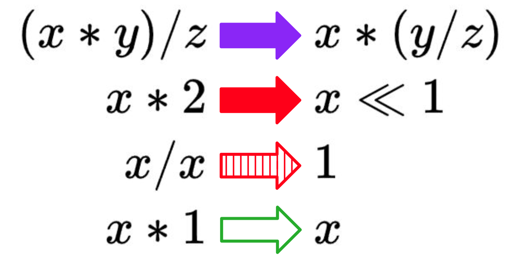
and our rewrite rules for it will be:
(x * y) / z => x * (y / z)
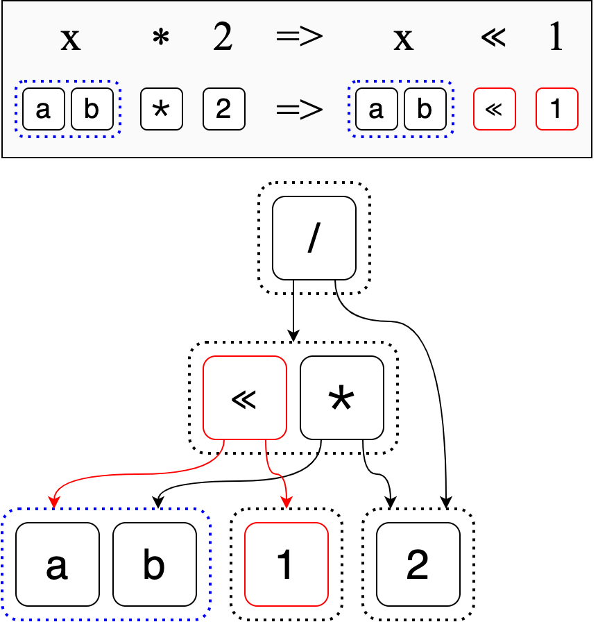
x * 2 => x << 1
x / x => 1
x * 1 => x
Here they are as an image. The arrows are visually different because they will be used to identify which rewrites apply in subsequent examples.
A naive solution
A naive approach to optimizing this expression is to look for a rewrite that applies, apply it, and repeat until we can’t find any other rewrites. What happens if multiple rewrites apply? Well I did say this was the naive solution, so in this case we can just pick randomly.
There are two possible rewrite paths for our example, but only one leads to the optimal expression.
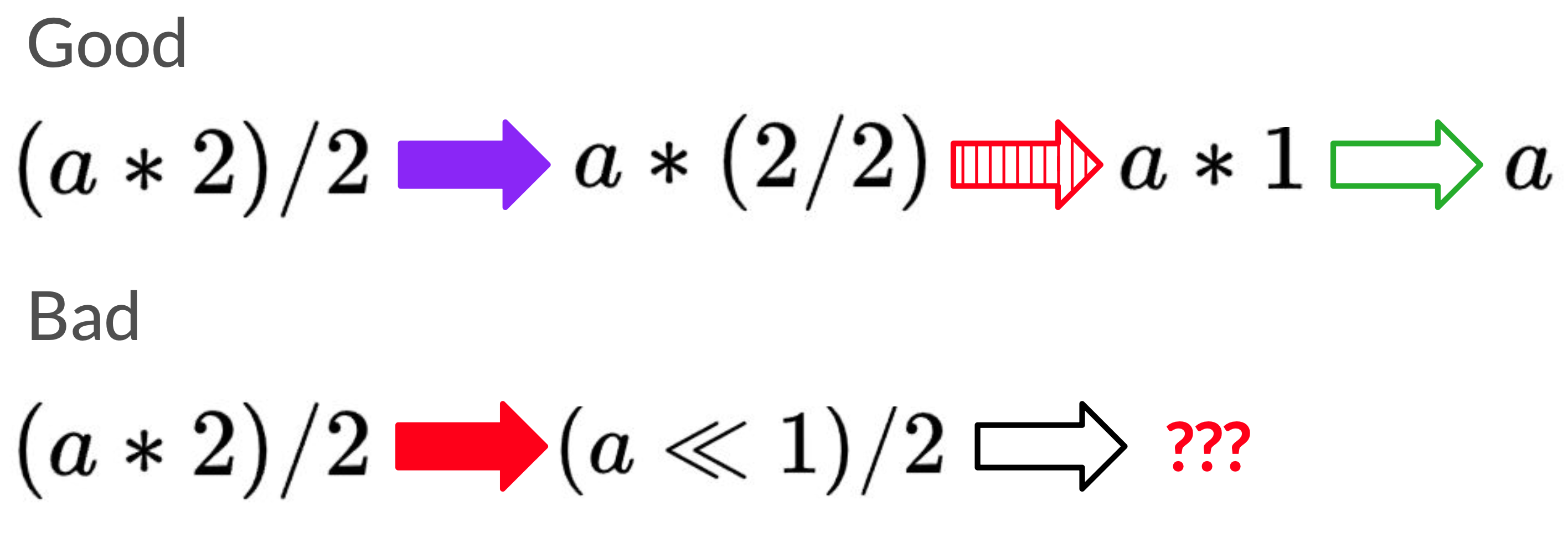
The bad rewrite path gets stuck at (a << 1) / 2, which there are no rewrites
out of. But how could we have known that this would lead to a dead end?
Well, in general it’s hard to know which rewrite is the correct rewrite to pick when we want the best of all possible expressions. Some rewrites might look like they’re bad or useless and eventually lead to the best expression and some might look great but leave us stuck with an inferior expression.
A less naive solution
From here on forward, we are not going to compromise on optimality. Let’s consider another naive, but complete solution (“complete” in the sense that it will always find the optimal expression).4
We will now add a list that tracks expressions equal to our input expression. This list will start just containing the input expression.
We will loop over each expression p in the list. We will then add to our list
each expression q that can be created by rewriting p. We’ll only add an expression
if it isn’t in the list already.
Here’s a gif of how the algorithm will proceed for our input.5
Once this process is done, our list will have every possible rewritten expression in it. (Not convinced? Read this footnote 6)
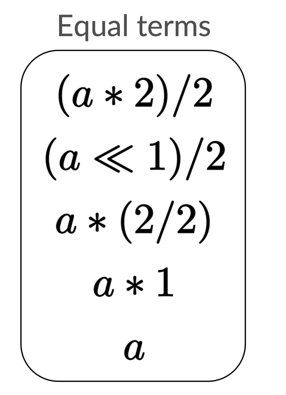
We can now take one last pass through this list and find the best (shortest)
expression, which is a.
Our answer is no longer beholden to lucky guesses, but this comes at a cost. Take a second to see if you can think of a starting expression and rewrites that make the equality list take up a lot of space (without making the algorithm infinitely loop).
It might not be so evident with our simple example, but if you often have multiple rewrites that apply to a given expression (even from the same rewrite rule), there will be an exponential number of expressions you can generate from your rewrite rules. Some may be duplicates, but not all.
For example, if we knew that a was equal to b and thus added the rewrite
rule
a => b
we would double the size of our equality list.
We could double it again by adding a => c, and if we repeated this process it
would only take a small number of rewrites to completely blow up our list.
The first optimization: sharing
Our current solution always finds the best expression but is naive because there might be too many expressions to store in its equality list. In these next two subsections I’m going to discuss how we can change our data structure to cut down on storage space. We’ll see later how to accommodate these changes and improve the overall algorithm.
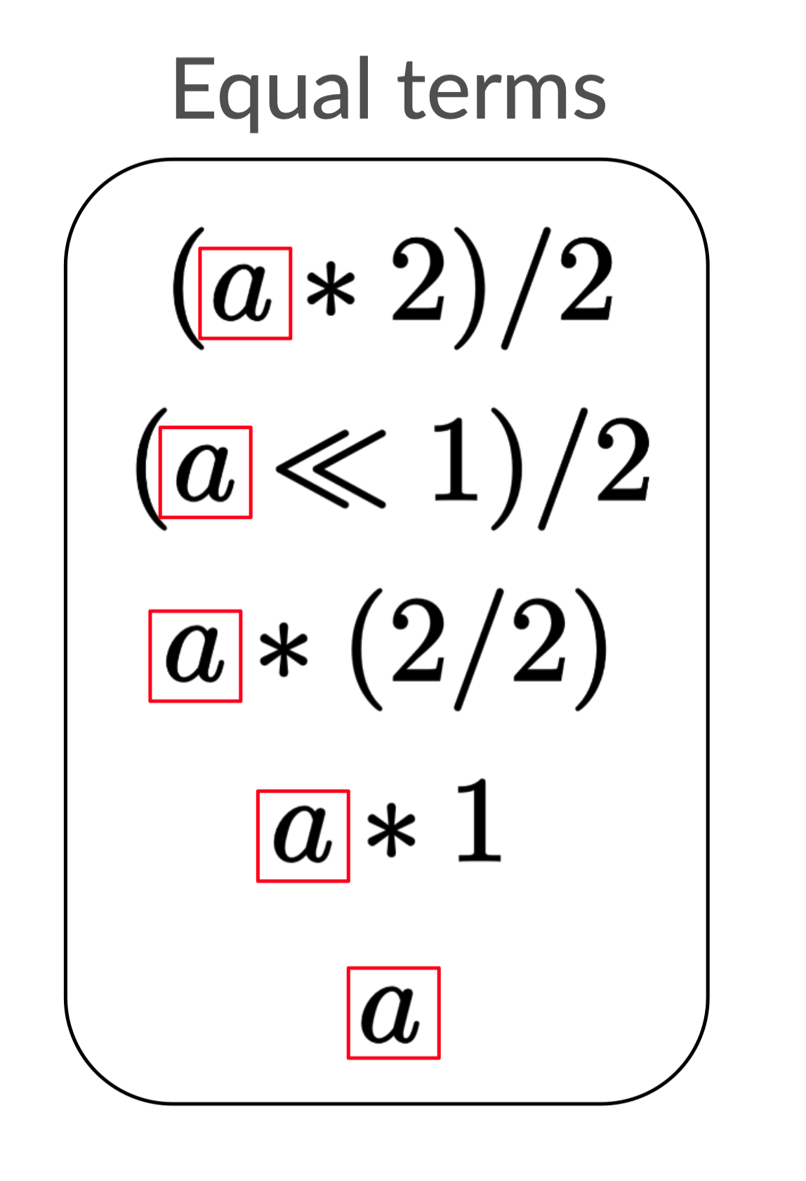
What we will do is exploit symmetries in our equality list (reproduced below) to make it more compact. Can you think of anything that feels redundant?
The first observation I’ll make is that many of the expressions have similar
structures. For example: a is present in each expression.
As David Byrne said
years ago, “Say something once, why say it again?” We can be clever here and
point every redundant occurrence to one. Then we only need to store a once!
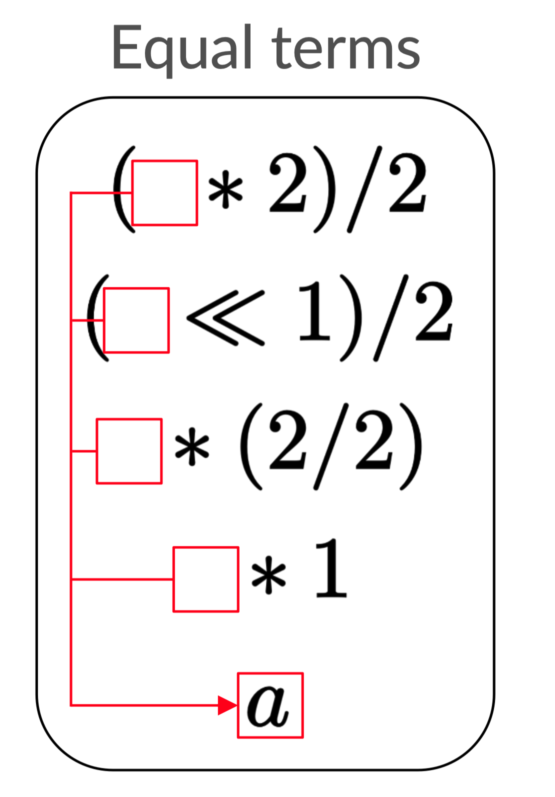
I refer to this optimization as “sharing” because the value a is shared among
many expressions. For demonstrative purposes, I only depicted one shared
expression, but in general it makes sense to share as much as you can.
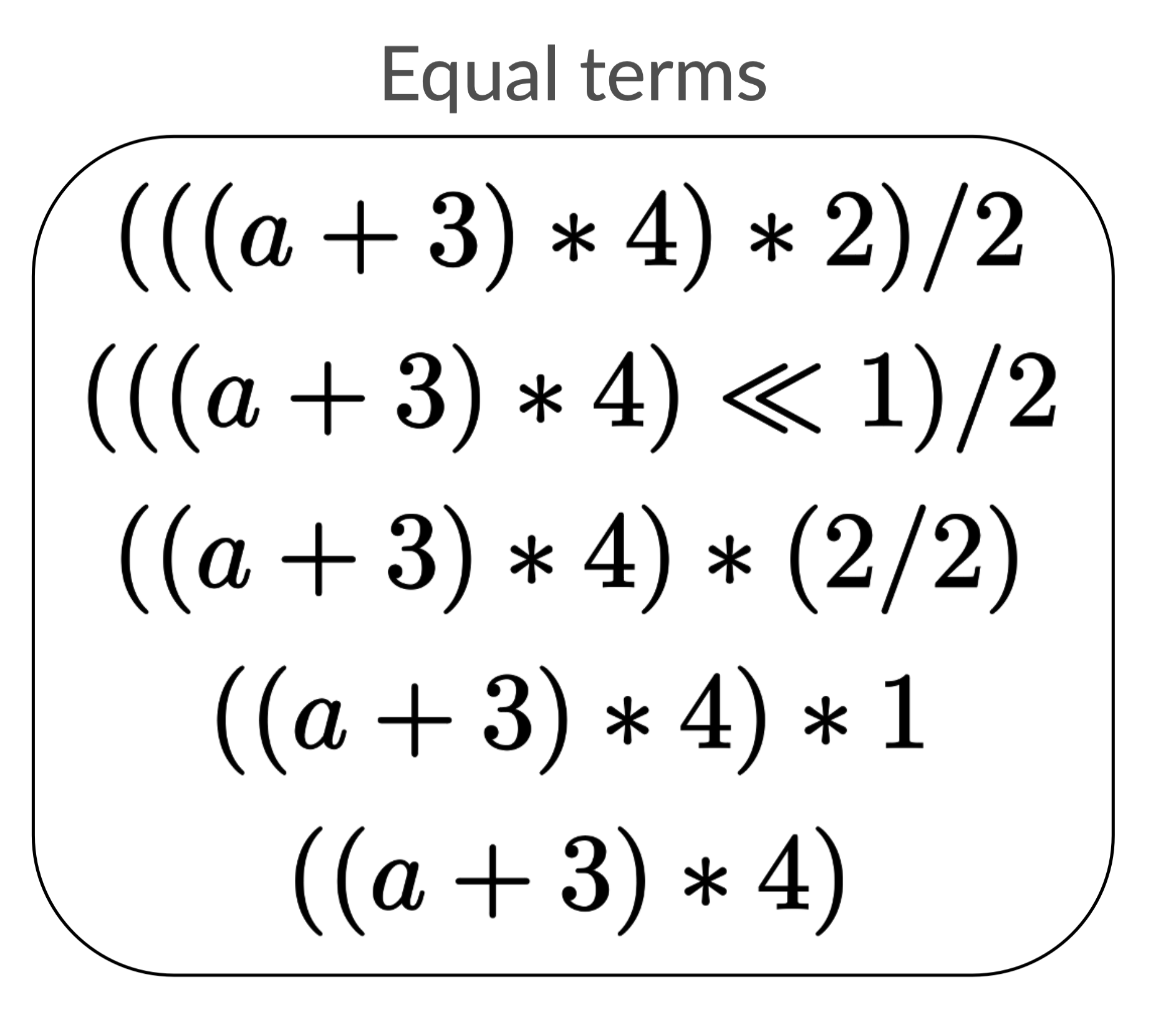
Now you might object that for this example it doesn’t look like we’ve really
made the expressions smaller. This is fair, but that’s only because our example
is on a small expression. We can see more immediate gains if a were instead
something like (a + 3) * 4.
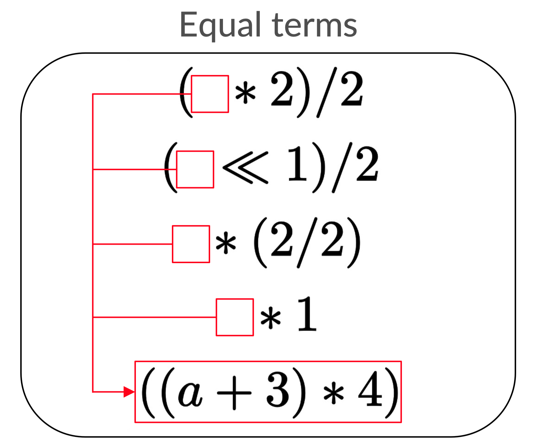
Sharing just (a + 3) * 4 is already a pretty big reduction.
The second optimization: semantic equality
Sharing helps us keep down on the size, but not number of expressions. Even if each expression is small, our list can still be huge because in a worst case there are exponentially many expressions.
Let’s return to the version of our example where we added the rewrite a => b.
If a and b were very large, sharing could reduce space,
but the number of expressions would still stay the same.
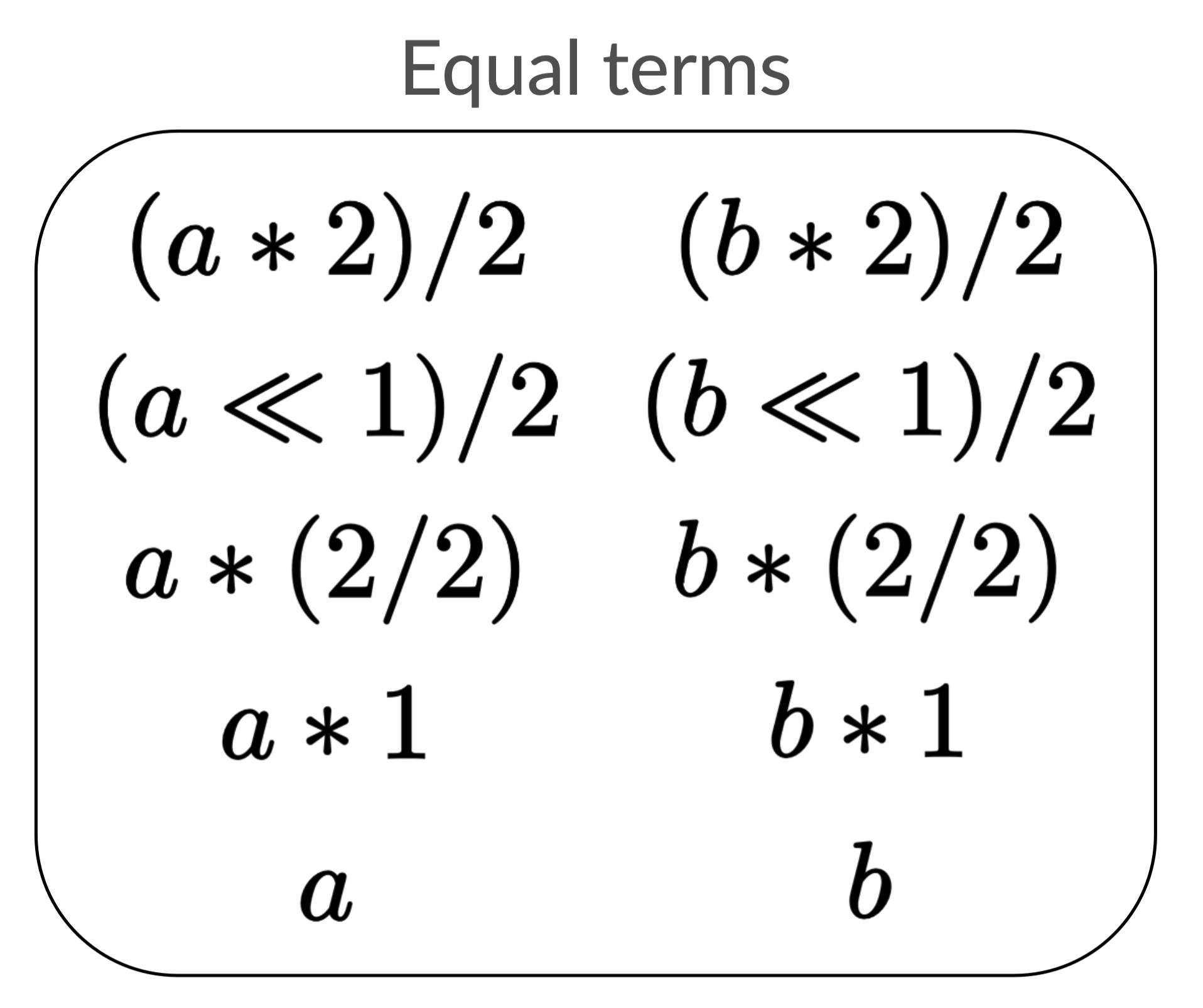
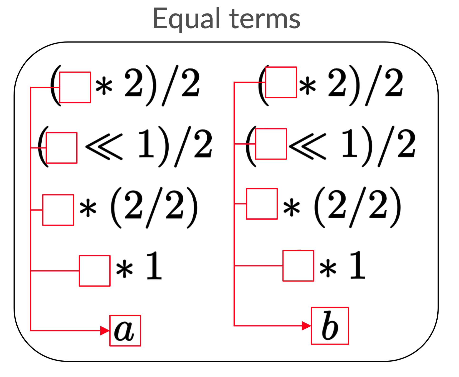
Look at the left and right columns of the list. These expressions are vexingly
similar to each other! Wouldn’t it be nice if we could somehow write the ( * 2)/2 part only once?
Why do we have this problem? Right now our optimizations are purely syntactic. We only share syntactically equal sub-expressions. We have another optimization, the uniqueness condition on adding expressions to the list, but this also only checks for syntactic equality.
However, our rewrite rules tell us about semantic equality. a and b are
not literally the same term, but our rewrite rule says that they are equal.
Our next insight will be to enforce semantic equality in our data structure through something known as equality classes.
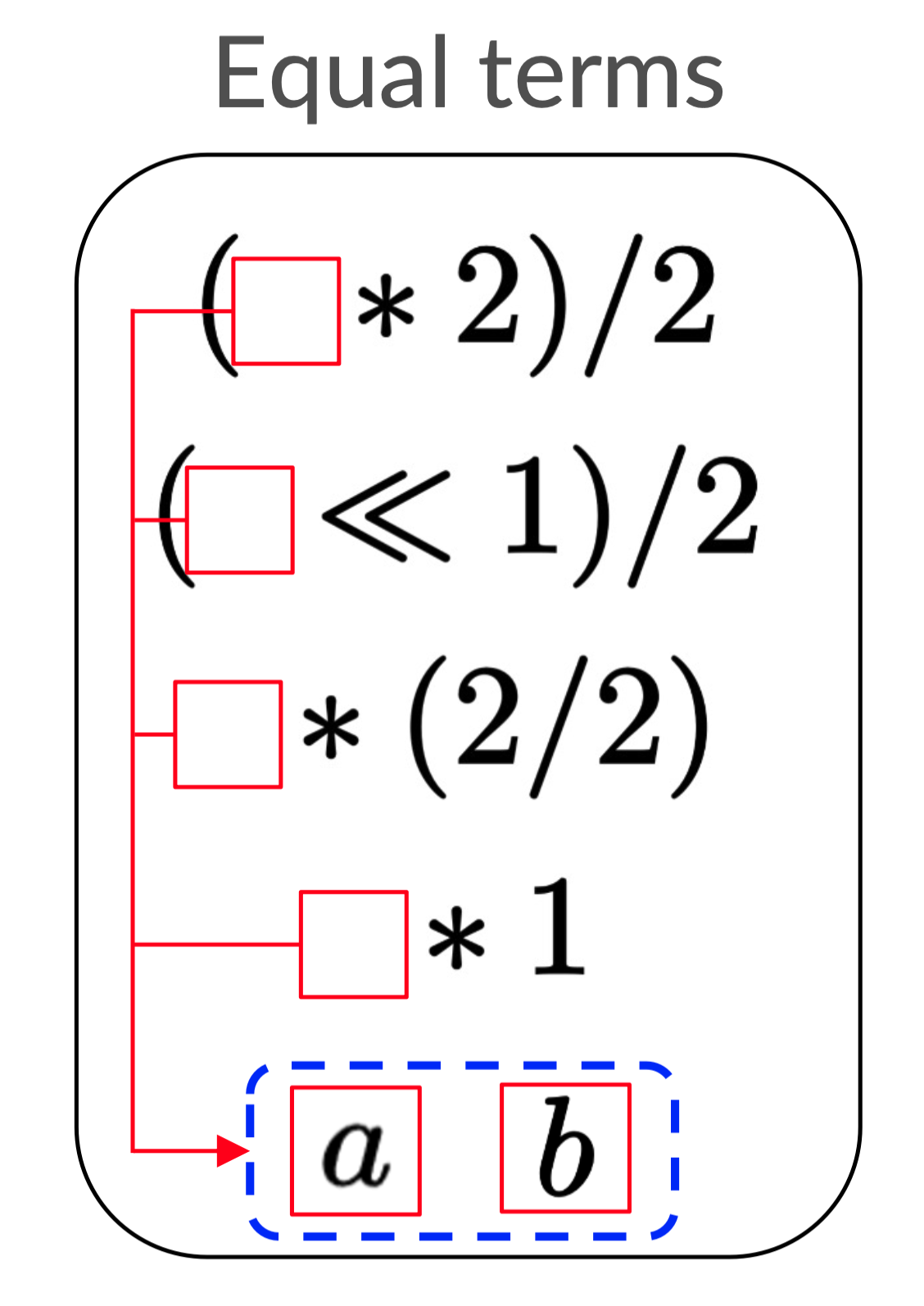
Each equality class (denoted by the dashed lines) contains elements which are
semantically equal according to our rewrite rules. Now (□ * 2) / 2 in our list
says precisely that □ can be either a or b!
Section 2: The e-graph
You may have observed that the equality list from the naive solution started to look less and less like a list as we optimized it. If we add all of the sharing and semantic equality optimizations, we end up with an e-graph. You’re finally ready to understand how this mess of arrows and dashed lines works.
First I’ll walk you through how to read this and other e-graphs, then I’ll give an idea of how to use an e-graph to solve the previous optimization problem.
Reading an e-graph
It’s not just because I was lazy that I avoided applying all of the optimizations to the examples in the previous section. E-graphs are really good at storing a lot of expressions compactly, but this also makes them difficult to read. I’ll try to build some intuition on how you can read one in this section.
Simple e-graphs
In the extreme case where an e-graph does not encode many expressions, it looks similar to an AST. (Don’t know what an AST is? Read this footnote 7)
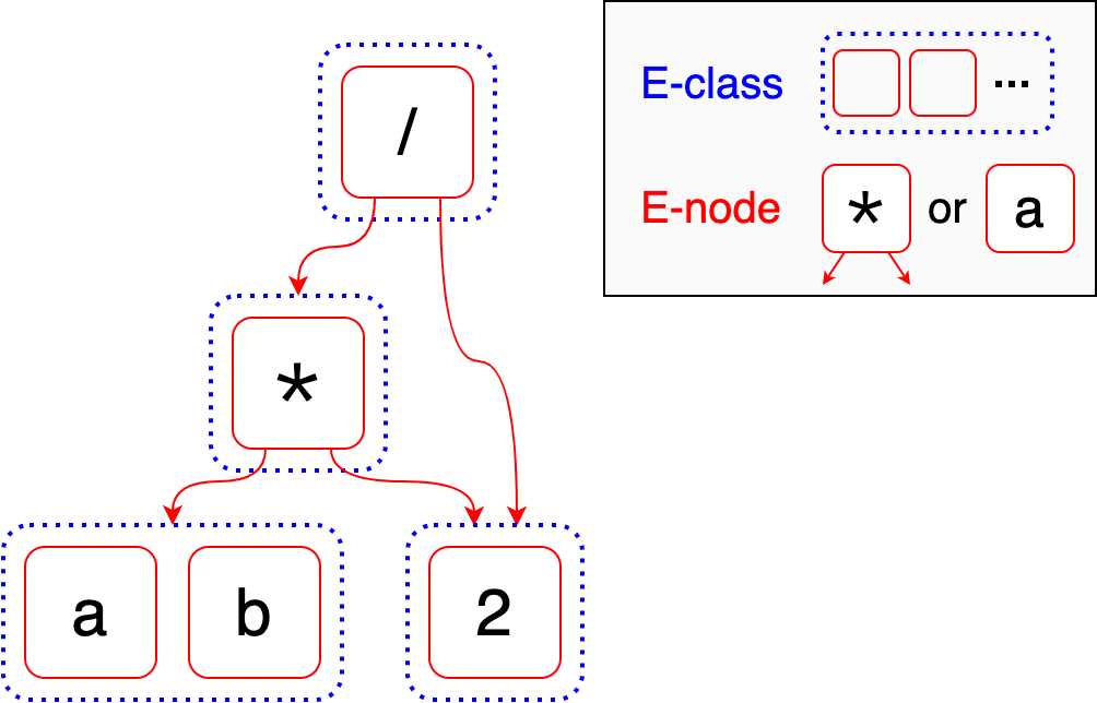
Equality nodes (e-nodes) are the terms in boxes like * or a. E-nodes
behave like the nodes in an AST: they can be values which have no arguments
(like a and 2) or operators which have arguments (like * and /). For
example, the * e-node has two arguments: first, the e-class containing a and
b, second, the e-class containing 2. The order of the arguments usually
matters.
Equality classes (e-classes) are the dashed containers. An e-class is a set
containing e-nodes which we know are equal. Most of the e-classes in this
example are an extreme case: they only have one value. However, the e-class on
the bottom left contains both a and b, which should be familiar from the
previous example.
Notice how when I was introducing e-nodes, I was careful to say an e-node’s
argument was “the e-class containing …” instead of referring to specific
e-nodes like a or 2. This is how we exploit semantic equality. Unlike in an
AST, e-nodes do not have other e-nodes as their arguments: they have e-classes
as arguments.
In the above example, the e-graph represents both (a * 2) / 2 and (b * 2) / 2
because the left argument of * is the e-class containing both a and b.
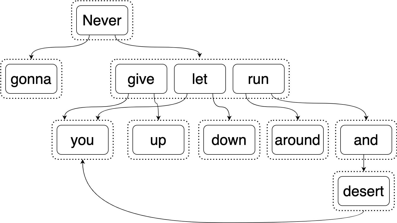
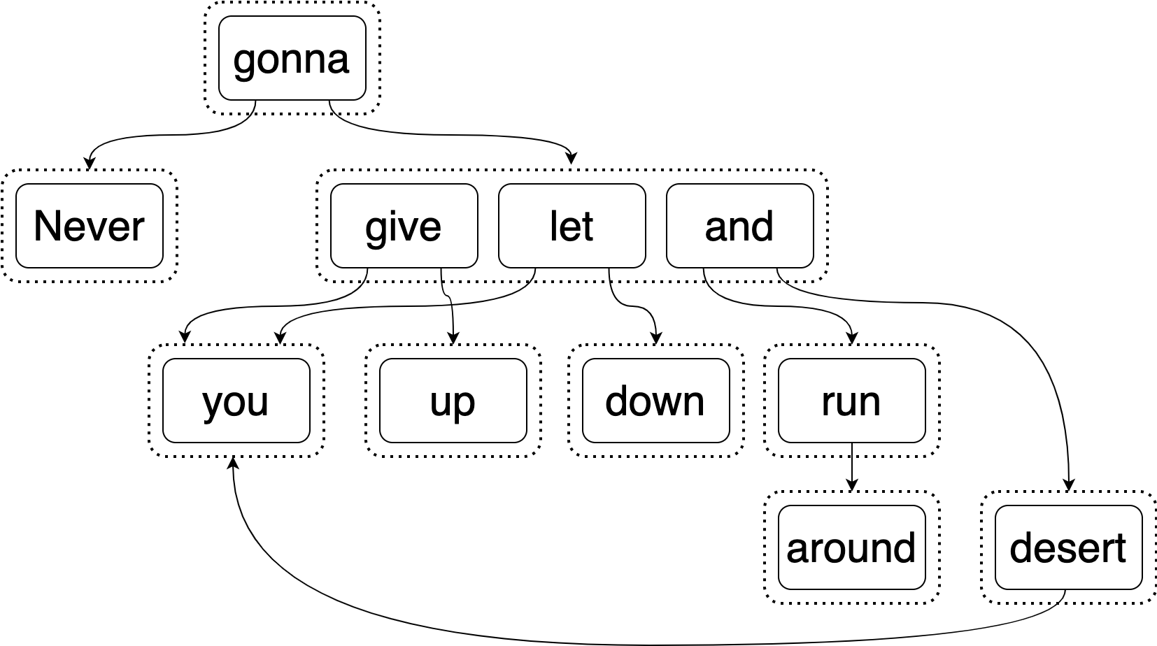
Equipped with this knowledge, you should be prepared to list off all of the expressions in what I refer to as the AstlE-Graph, which contains some of the things which Rick Astley will equivalently (not) do. (Do things look like they’re in the wrong order? Read this footnote 8)
Cycles
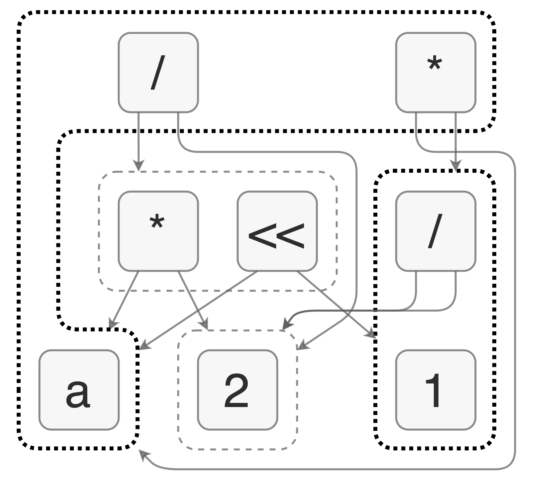
So far our examples have all looked kind of like trees (really, DAGs). But e-graphs can have cycles too. Can you guess the equivalent expressions represented by the following e-graph?
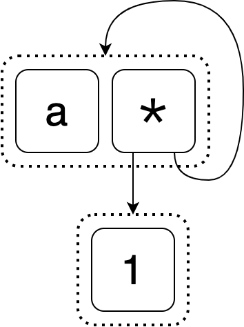
The first is a. The next one is trickier. It starts out 1 * □. For the □
we get to choose from a and 1 * □. If we picked a, we would get 1 * a.
If we picked 1 * □, we would now have 1 * 1 * □ and we would once again have
to make the same choice between a and 1 * □ to figure out what to fill in
for □. This proceeds forever: this 3 element e-graph represents infinitely
many equal expressions!
E-graph operations
In this section I’ll describe the main operations in an e-graph. I’ll give you a simplified picture of how they work, so be mindful that there might be more going on under the hood in a real implementation.
Adding
When we built the equality list in the naive solution, adding a new expression was easy. If it wasn’t in the list already, we added it. E-graphs are much more compact than a list, and as a result adding expressions to them is more complicated.
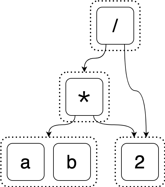
Let’s start with an intial e-graph that represents the starting expression (a * 2) / 2.
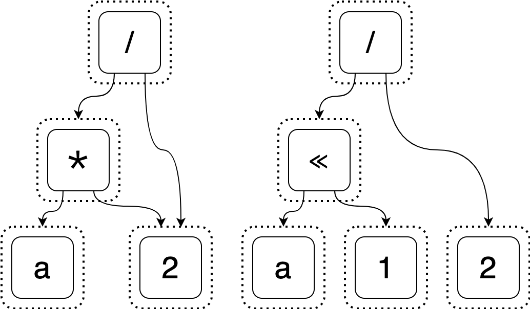
Suppose we’ve discovered that (a * 2) / 2 is equal to (a << 1) / 2 and want
to add it. The simplest way to do this would be to create several new e-classes
for this expression just like how we represented the initial expression.
You should hopefully object to this - this is not very compact at all! We aren’t done yet, though. If we stopped here, we wouldn’t be taking advantage of sharing. If one of the e-nodes we add is the exact same as an existing e-node, we’ll instead share the existing one.

This is closer, but we still aren’t done. Let’s not forget our second optimization: we know that the new expression is semantically equal to the initial one, so we shouldn’t just keep their roots in separate e-classes.
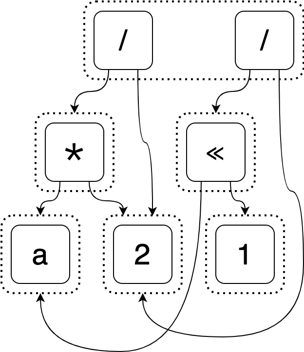
This is good, but it turns out it can be even better! The e-graph below is a more compact version.9 Take a second to convince yourself that this e-graph still represents the same equalities as the one before it.
But even the “naive” way of adding expressions lets us store many more expressions than would be feasible in the equality list we were using. We will see in the next section how we can improve both our algorithmic performance and obtain the more compact e-graph.
Directly applying rewrites
I’ve been implying that we would improve our naive optimization algorithm by swapping the equality list in it with an e-graph. However, there’s a problem with doing this. The algorithm would still loop over each expression we want to add to the e-graph - yes, we can now store all of them, but it’s easy to make the number of expressions (and thus, iterations) really large.
It’s about time we revisit how we’re generating new expressions. Up ’til now, we would take a single expression and find the ways we could apply our rewrite rules to make new ones. We saw in the previous section how we could then add those new expressions to the e-graph. It turns out that we can skip to applying rewrites directly to the e-graph - and also that doing this helps keep down the size of the e-graph!
Let’s say we start with the e-graph to representing both (a * 2) / 2 and
(b * 2) / 2
and we want to apply the rewrite rule
x * 2 => x << 1
The naive approach would be to iterate over both (a * 2) / 2 and (b * 2) / 2, apply the rewrite to produce (a << 1) / 2 and (b << 1) / 2
respectively, and add each expression to the e-egraph. In total, we would have
two iterations and two expressions to add.
You saw in the previous section how adding (a << 1) / 2 worked. We’d have to do
all that work again for (b << 1) / 2.
Instead, let’s apply the rewrite directly to the e-graph. What this means is
that we will match x not to a concrete term, but to an e-class. Specifically, x
will match to the e-class which contains a and b.
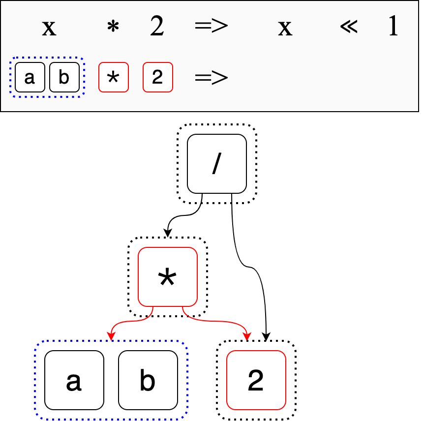
Then we can perform the rewrite directly on the e-graph.
Observe how we don’t have to first rewrite our inital expressions, then add the
two new expressions (a << 1) / 2 and (b << 1) / 2. We directly put x << 1
into the same e-class as x * 2. And the e-graph is the smaller form we
couldn’t obtain in the previous section.
Applying the rewrite directly has several benefits. First, a single rewrite can produce multiple equivalent expressions. Second, the rewrite is local, meaning it makes small changes to the e-graph instead of creating an entirely new expression and then adding it to the e-graph. Finally, the e-graph it creates is much more compact than the one we would get by naively adding whole expressions, because we can reason more about equality on a local scale.
Extraction
I’ve described how to change our naive algorithm first to compactly store its search space using an e-graph, and then to reduce its search time by applying rewrites to the e-graph directly.
Unfortunately, once we have applied all the rewrites that we can to our e-graph, we no longer have an easy way of listing off expressions to find the best one. Because our e-graphs can represent so many equivalent expressions, it isn’t in our interest to list them all off either!
Instead, we now must traverse the e-graph to find the best expression in a process known as “extraction.” You provide some heuristic for evaluating expressions (such as size) and the extraction algorithm will go and find the best expression using your heuristic.
This is where I reveal that I’ve been lying to you a bit. Extraction in popular libraries, such as egg, is done using a greedy algorithm. So we might end up compromising on the best expression. It turns out that the extraction problem is NP-complete.
In practice, I’ve found extraction to not be the limiting factor in performance or quality when using e-graphs. Perhaps things break down in edge cases I have yet to encounter.
Fin
That’s e-graphs in a nutshell!
My hope is that you’re now familiar enough to identify where using an e-graph might help your own work. (If you found this helpful, that makes me overjoyed!)
Additional reading
My introduction to e-graphs was egg, which adds several improvements to the data structure as well as a nice implementation in Rust. E-graphs have been around for a while, but in my view egg has helped to (re)popularize them.
Readers have suggested some other references, which I’m including below (Have a suggestion? Feel free to reach out):
- Cranelift is using e-graphs, see this
RFC
for details
- Also suggested: Chris Fallin’s presentation on this work.
- Philip Zucker has a blog post about implementing e-graphs in Julia and a follow-up post on doing pattern matching in them. These go into more details on their workings.
- The folks behind egg have been hosting an EGRAPHS workshop for a few years now. That link goes to the 2023 one, which should point back to previous editions.
- egglog is as far as I understand intended to be the successor of egg, combining it and datalog.
Credits
My primary credit is egg (mentioned above). I stole the first e-graph diagram from egg, as well as the example expression and rewrite rules.
Many thanks as always to the myriad friends who gave feedback on this post.
Comments
I don’t do any fancy stuff with comments on my website. You can reach out to me or leave a comment on:
-
I am partial to code golfing after all. ↩︎
-
We will not check that the rewrite rules actually yield equal expressions - it is up to the user to provide correct rewrite rules. ↩︎
-
We have a rewrite rule that says “if you have something that looks like
x * 1, you can replace it withx”. We start with the expression(a + (3 * 1)) * 1.Take a second to see which parts of the expression you can find that look like
x * 1.There are two sub-expressions that look like
x * 1:3 * 1(wherex = 3) and(a + (3 * 1)) * 1(wherex = (a + (3 * 1))).I’m choosing to start with the
3 * 1expression. We can replace it by3, resulting in(a + 3) * 1Then we can repeat this process with the last match,
(a + 3) * 1, to get
↩︎a + 3 -
I don’t want to make the claim that the best way to solve this problem is to be uncompromising about your solution’s completeness. There will surely be problems for which it is helpful to use randomness to narrow your search space. Requiring a complete solution is pedagogically helpful here (partly because e-graphs are good at this!). ↩︎
-
You’ll note that it says “Equal terms” instead of “Equal expressions” - that’s just for brevity and I use the two words interchangeably. ↩︎
-
We’ll show this by contradiction. Suppose there was a rewritten expression
qthis algorithm didn’t consider. Then there must be someq1such thatq1rewrites intoq. Ifq1was in the algorithm’s equality list, thenqmust have been added (this is part of the algorithm). Otherwise, we reason there must be aq2such thatq2rewrites intoq1and repeat this process onq2. Since our rewrite “path” must be finite (otherwise the algorithm wouldn’t terminate), we’ll eventually be able to follow it all the way back to the starting expression. The starting expression can’t be in our list because it would imply that we eventually addq. But this is a contradiction because we require that the starting expression is in our list. ↩︎ -
So far when I’ve been putting expression into our equality list, they’ve been strings.
(a * 2) / 2is just a sequence of characters.It turns out that a sequence of characters is not the most useful form for representing an expression. An abstract syntax tree, or AST, is a way of encoding the expression structure in a more tractable form.
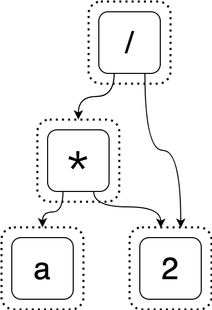
Here’s an example of the AST for
(a * 2) / 2.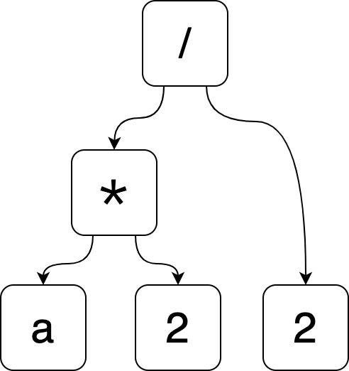
I think the most confusing part about ASTs is how the two higher nodes (
*and/) work. It should be pretty obvious that the nodes on the bottom are just the valuesa,2, and2again.Let’s first look at the
*node. Informally, this node says, “My operation is*. My first argument isaand my second argument is2”. In this context,*mean multiplication, so this node represents the product ofaand2. If we wrote it out as a string, we would writea * 2.Can you interpret the
/node now? The only tricky thing about this node is that its first argument is another operation node. This node says, “My operation is/. My first argument is the*node (which representsa * 2) and my second argument is2.” If we were to write this node out as a string, it would be(a * 2) / 2.Notice how there aren’t any parentheses in the AST, but I have to put them in the string for clarity? That’s part of what is helpful about using an AST: it’s explicit what order operations go in. ↩︎
-
So far the examples we’ve been working with have had infix nodes like
*. We generally don’t think of it as being prefix like* a 2. The AstlE-Graph, however, has its operation nodes read in prefix, so you’d read the top node as being “Never gonna _”.Really there is no requirement on what order you parse an e-graph (or an AST) as long as you’re consistent - in some ways this order is only required for parsing and printing expressions from the data structure.
I originally had the following e-graph which I created using a bastardization of the kind of syntax tree linguists would write.
As an exercise, can you work out why I didn’t choose to have the operation nodes in the AstlE-Graph be in infix? I could’ve done that to be consistent with my other examples, but I chose not to. ↩︎
-
Originally, I falsely claimed that we could continue performing simplifications to end up with this compact e-graph, but that is false, as pointed out by dpercy. ↩︎